Simulating The Double Pendulum Using Lagrangian Formulation
The double pendulum is a classic example of a chaotic system in physics. It consists of two pendulums of \( L_1 \) and \( L_2 \) attached end to end, and its motion is highly sensitive to initial conditions. In this project, we will simulate the motion of a double pendulum using the Lagrangian formulation and visualize the results using Python's Matplotlib library.
The position of the masses can be described using the angles \( \theta_1 \) and \( \theta_2 \), which represent the angles of the first and second pendulums with respect to the vertical axis. Then the position of the masses can be expressed as: \[ x_1 = L_1 \sin\theta_1, \quad y_1 = -L_1 \cos\theta_1, \quad x_2 = x_1 + L_2 \sin\theta_2, \quad y_2 = y_1 - L_2 \cos\theta_2 \] The Kinetic Energy of the system is given by: \[ T = \frac{1}{2} m_1 ( \dot{x}_1^2 + \dot{y}_1^2 ) + \frac{1}{2} m_2 ( \dot{x}_2^2 + \dot{y}_2^2 ) \] The Potential Energy of the system is given by: \[ V = m_1 g y_1 + m_2 g y_2 = - m_1 g L_1 \cos\theta_1 - m_2 g (L_1 \cos\theta_1 + L_2 \cos\theta_2) \] The Lagrangian \( \mathcal{L} \) is defined as the difference between the Kinetic and Potential Energies: \[ \mathcal{L}(\theta_1, \theta_2, \dot{\theta}_1, \dot{\theta}_2) = T - V \] From Euler-Lagrange equations, we derive the equations of motion for the double pendulum: \[ \frac{d}{dt} \left( \frac{\partial \mathcal{L}}{\partial \dot{\theta}_i} \right) - \frac{\partial \mathcal{L}}{\partial \theta_i} = 0, \quad i = 1, 2 \]
Necessary Packages and Paths
    import numpy as np
    from scipy.integrate import solve_ivp
    import matplotlib.pyplot as plt
    from matplotlib.animation import FuncAnimation
Initial Setup
    g = 9.81          # gravitational acceleration (m/s^2)

    L1 = 0.75          # length of first rod (m)
    L2 = 1.25          # length of second rod (m)

    m1 = 2.0          # mass of first bob (kg)
    m2 = 1.0          # mass of second bob (kg)

    theta1_0 = np.pi/2       # initial angle of first pendulum (rad)
    theta2_0 = np.pi/2 + 0.1 # initial angle of second pendulum (rad)

    omega1_0 = 0.0           # initial angular velocity of first pendulum (rad/s)
    omega2_0 = 0.0           # initial angular velocity of second pendulum (rad/s)
Simulation Setup
    t_start = 0.0
    t_end   = 20.0
    dt      = 0.01
    t_eval  = np.arange(t_start, t_end, dt)
Simulation
    def double_pendulum_rhs(t, y, L1, L2, m1, m2, g):
        theta1, omega1, theta2, omega2 = y

        delta = theta2 - theta1

        den1 = (m1 + m2)*L1 - m2*L1*np.cos(delta)*np.cos(delta)
        den2 = (L2/L1) * den1

        # Angular accelerations
        num1 = (m2*L1*omega1*omega1*np.sin(delta)*np.cos(delta) +
                m2*g*np.sin(theta2)*np.cos(delta) +
                m2*L2*omega2*omega2*np.sin(delta) -
                (m1 + m2)*g*np.sin(theta1))

        alpha1 = num1 / den1

        num2 = (-m2*L2*omega2*omega2*np.sin(delta)*np.cos(delta) +
                (m1 + m2)*(g*np.sin(theta1)*np.cos(delta) -
                        L1*omega1*omega1*np.sin(delta) -
                        g*np.sin(theta2)))

        alpha2 = num2 / den2

        return [omega1, alpha1, omega2, alpha2]
Solving ODEs
    y0 = [theta1_0, omega1_0, theta2_0, omega2_0]

    sol = solve_ivp(
        double_pendulum_rhs,
        t_span=(t_start, t_end),
        y0=y0,
        t_eval=t_eval,
        args=(L1, L2, m1, m2, g),
        rtol=1e-9,
        atol=1e-9
    )

    theta1 = sol.y[0]
    omega1 = sol.y[1]
    theta2 = sol.y[2]
    omega2 = sol.y[3]
Position
    x1 = L1 * np.sin(theta1)
    y1 = -L1 * np.cos(theta1)

    x2 = x1 + L2 * np.sin(theta2)
    y2 = y1 - L2 * np.cos(theta2)
Compute Angular Acceleration
    def compute_angular_accelerations(theta1, omega1, theta2, omega2):
        alpha1 = np.zeros_like(theta1)
        alpha2 = np.zeros_like(theta2)
        for i in range(len(theta1)):
            _, a1, _, a2 = double_pendulum_rhs(
                t_eval[i],
                [theta1[i], omega1[i], theta2[i], omega2[i]],
                L1, L2, m1, m2, g
            )
            alpha1[i] = a1
            alpha2[i] = a2
        return alpha1, alpha2

    alpha1, alpha2 = compute_angular_accelerations(theta1, omega1, theta2, omega2)
Compute Linear Velocity
    vx1 = L1 * omega1 * np.cos(theta1)
    vy1 = L1 * omega1 * np.sin(theta1)

    vx2 = vx1 + L2 * omega2 * np.cos(theta2)
    vy2 = vy1 + L2 * omega2 * np.sin(theta2)
Final Values
    def numerical_derivative(f, t):
        df = np.zeros_like(f)
        df[1:-1] = (f[2:] - f[:-2]) / (t[2:] - t[:-2])
        df[0] = (f[1] - f[0]) / (t[1] - t[0])
        df[-1] = (f[-1] - f[-2]) / (t[-1] - t[-2])
        return df

    ax1 = numerical_derivative(vx1, t_eval)
    ay1 = numerical_derivative(vy1, t_eval)
    ax2 = numerical_derivative(vx2, t_eval)
    ay2 = numerical_derivative(vy2, t_eval)

    x1_mag = x1
    v1_mag = np.sqrt(vx1**2 + vy1**2)
    a1_mag = np.sqrt(ax1**2 + ay1**2)

    x2_mag = x2
    v2_mag = np.sqrt(vx2**2 + vy2**2)
    a2_mag = np.sqrt(ax2**2 + ay2**2)
Animation
    fig_anim, ax_anim = plt.subplots(figsize=(5, 5))
    ax_anim.set_aspect('equal')
    max_len = L1 + L2
    ax_anim.set_xlim(-max_len*1.1, max_len*1.1)
    ax_anim.set_ylim(-max_len*1.1, max_len*1.1)
    ax_anim.set_xlabel('x ($m$)')
    ax_anim.set_ylabel('y ($m$)')

    line, = ax_anim.plot([], [], 'o-', lw=2, color = '#363636')
    trace, = ax_anim.plot([], [], '-', lw=1, alpha=0.5, color = '#DB4437')
    time_text = ax_anim.text(0.05, 0.9, '', transform=ax_anim.transAxes)

    # Keep a trace of the second bob
    trace_x, trace_y = [], []

    def init():
        line.set_data([], [])
        trace.set_data([], [])
        time_text.set_text('')
        return line, trace, time_text

    def update(frame):
        # Current positions
        this_x = [0, x1[frame], x2[frame]]
        this_y = [0, y1[frame], y2[frame]]
        line.set_data(this_x, this_y)

        trace_x.append(x2[frame])
        trace_y.append(y2[frame])
        trace.set_data(trace_x, trace_y)

        time_text.set_text(f't = {t_eval[frame]:.2f} s')
        return line, trace, time_text

    anim = FuncAnimation(
        fig_anim,
        update,
        frames=len(t_eval),
        init_func=init,
        interval=dt*1000,
        blit=True
    )
    anim.save('double_pendulum.mp4', fps=30, dpi=150)
Output Animation
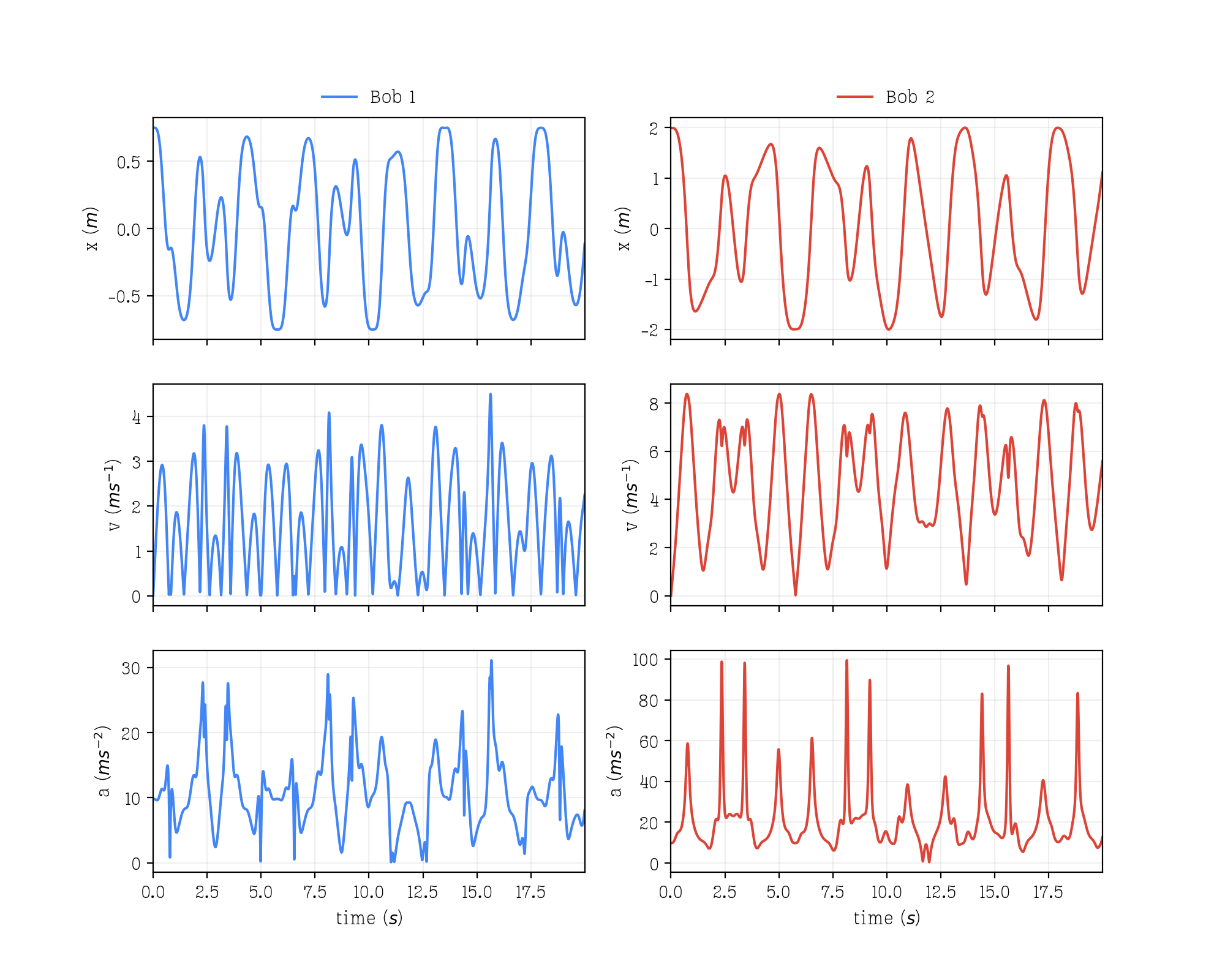
Plotting
    fig, axes = plt.subplots(3, 2, figsize=(10, 8), sharex=True)

    # Bob 1
    axes[0, 0].plot(t_eval, x1_mag, label='Bob 1', color = '#4285F4')
    axes[0, 0].set_ylabel('x ($m$)')
    axes[0, 0].legend(loc='upper center', bbox_to_anchor=(0.5, 1.2), ncol=1, frameon=False)
    axes[0, 0].grid(alpha=0.2)
    axes[0, 0].set_xlim([t_eval[0], t_eval[-1]])

    axes[1, 0].plot(t_eval, v1_mag, color = '#4285F4')
    axes[1, 0].set_ylabel('v ($ms^{-1}$)')
    axes[1, 0].grid(alpha=0.2)
    axes[1, 0].set_xlim([t_eval[0], t_eval[-1]])

    axes[2, 0].plot(t_eval, a1_mag, color = '#4285F4')
    axes[2, 0].set_ylabel('a ($ms^{-2}$)')
    axes[2, 0].set_xlabel('time ($s$)')
    axes[2, 0].grid(alpha=0.2)
    axes[2, 0].set_xlim([t_eval[0], t_eval[-1]])

    # Bob 2
    axes[0, 1].plot(t_eval, x2_mag, color = '#DB4437', label='Bob 2')
    axes[0, 1].set_ylabel('x ($m$)')
    axes[0, 1].legend(loc='upper center', bbox_to_anchor=(0.5, 1.2), ncol=1, frameon=False)
    axes[0, 1].grid(alpha=0.2)
    axes[0, 1].set_xlim([t_eval[0], t_eval[-1]])

    axes[1, 1].plot(t_eval, v2_mag, color = '#DB4437')
    axes[1, 1].set_ylabel('v ($ms^{-1}$)')
    axes[1, 1].grid(alpha=0.2)
    axes[1, 1].set_xlim([t_eval[0], t_eval[-1]])

    axes[2, 1].plot(t_eval, a2_mag, color = '#DB4437')
    axes[2, 1].set_ylabel('a ($ms^{-2}$)')
    axes[2, 1].set_xlabel('time ($s$)')
    axes[2, 1].grid(alpha=0.2)
    axes[2, 1].set_xlim([t_eval[0], t_eval[-1]])
    plt.savefig('DoublePendulum.png', dpi = 200)
    plt.show()
Simulation Result